Predicting the VIX
This notebook builds a probabilistic forecast for the VIX. Instead of predicting a single future value, we model the full distribution of possible changes in VIX, conditional on its current level. With that conditional distribution in hand, we can draw scenarios, compute prediction bands (fan charts), and summarize risk in a way that reflects how the VIX behaves differently in calm versus turbulent markets.
This notebook:
Loads daily VIX history and builds a series
x = log(CLOSE).Fits a 2D GMM on pairs
(x_t, x_{t+1} - x_t).Builds the conditional model \(p(x_{t+1} - x_t\mid x_t)\).
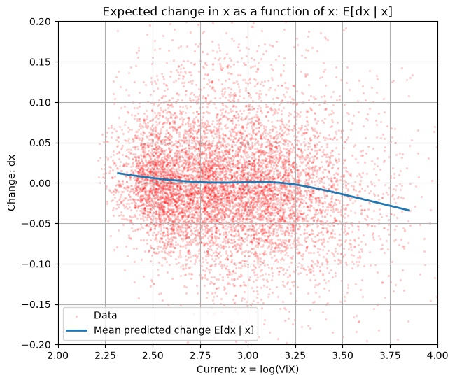
Plots the posterior mean function \(\mathbb{E}[x_{t+1} - x_t \mid x_t]\).
Simulates multi-step scenarios by iteratively sampling from the conditional.
Loading the VIX data
The code below reads the historical VIX series from file, parses the date column, and sets it as the time index so that later time-based operations behave correctly. It also standardizes column names and drops any rows with missing values, ensuring the dataset is clean and ready for transformations and modeling.
Loaded local CSV: data/VIX_History.csv
        DATE   OPEN   HIGH    LOW  CLOSE
0 1990-01-02  17.24  17.24  17.24  17.24
1 1990-01-03  18.19  18.19  18.19  18.19
2 1990-01-04  19.22  19.22  19.22  19.22
3 1990-01-05  20.11  20.11  20.11  20.11
4 1990-01-08  20.26  20.26  20.26  20.26
Compute x=log(VIX) and it's daily change
Here we transform the raw VIX level to log-space and compute its one-day change. Taking logs stabilizes the scale (large and small values become more comparable), and differencing the log series isolates day-to-day movements. The result is a target variable (the log change) and a conditioning variable (the log level) aligned on the same dates, with any initial NaN from differencing removed.
Fit a regression model
This section fits a simple regression of the daily log change on the current log level. The goal is to capture the average relationship-e.g., whether VIX tends to drift up or down depending on where it currently sits.
Fit a condtion model
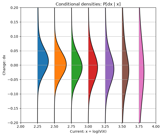
Now we fit the conditional distribution of the daily log change given the current log level using a Conditional Gaussian Mixture Model (CGMM). Instead of a single bell curve, the model represents the outcome as a mixture of Gaussians whose weights and parameters adapt with the conditioning variable. This lets the shape of the distribution change with the level-capturing skew, fat tails, and non-linearity that a plain regression can't. After training, we plot confitional densities of the next-day-chage, for different values of current level.
Monte Carlo path simulation
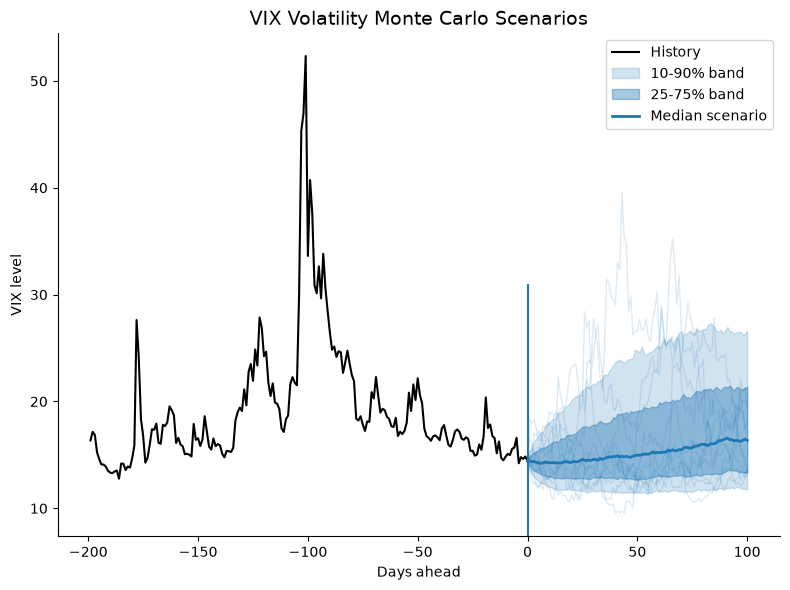
Using the fitted conditional model, we simulate many forward paths. Starting from today’s log level, each step draws a daily log change from the learned distribution conditional on the current level, updates the level, and repeats for the desired horizon. Converting back from log space yields VIX trajectories. Aggregating these paths produces a fan chart (e.g., median and 10-90% bands) that reflects both drift and state-dependent volatility and tail risk.
Gallery Image
fig, ax = plt.subplots(figsize=(8,6))

hist_n = 200
ax.plot(np.arange(-hist_n+1, 1), np.exp(x[-hist_n:]),
        color="k", lw=1.5, label="History")

q = np.quantile(vix_paths, [0.1, 0.25, 0.5, 0.75, 0.9], axis=0)
t = np.arange(H+1)
ax.fill_between(t, q[0], q[-1], color="tab:blue", alpha=0.2, label="10-90% band")
ax.fill_between(t, q[1], q[-2], color="tab:blue", alpha=0.4, label="25-75% band")
ax.plot(t, q[2], color="tab:blue", lw=2, label="Median scenario")

for i in range(min(10, N)):
    ax.plot(t, vix_paths[i], color="tab:blue", alpha=0.15, lw=1)

ax.set_xlabel("Days ahead")
ax.set_ylabel("VIX level")
ax.set_title("VIX Volatility Monte Carlo Scenarios", fontsize=14)
ax.axvline(x=0,ymin=0,ymax=.50)
ax.spines[['right', 'top']].set_visible(False)
ax.legend()
plt.tight_layout()
plt.savefig('gallery_images/vix.png', dpi=150, bbox_inches='tight')

plt.show()