Heavy-tailed & skewed conditional regression

Real residuals are often heavy-tailed (occasional large errors) and skewed (asymmetric). A Gaussian conditional model under-states the tails and cannot represent asymmetry. cgmm provides three drop-in conditional regressors that share the same API but differ in the family of the joint mixture they fit and then condition:

Regressor	Family	Captures
ConditionalGMMRegressor	Gaussian	mean, (co)variance
ConditionalStudentTRegressor	Student-t	+ heavy tails
ConditionalGHRegressor	Generalized Hyperbolic	+ skewness

See Distributions & Conditioning for the equations and the EM algorithms. Below we fit all three on synthetic data whose noise is both heavy-tailed and right-skewed, and compare their conditional densities and held-out log-likelihood.

import matplotlib
matplotlib.use('module://matplotlib_inline.backend_inline')  # capture figures inline (must be before pyplot import)
import numpy as np
import matplotlib.pyplot as plt
from scipy.stats import skewnorm, chi2

from cgmm import (
    ConditionalGMMRegressor,
    ConditionalStudentTRegressor,
    ConditionalGHRegressor,
)

rng = np.random.default_rng(7)

def make_data(n, seed, df=4, skew=6.0, scale=0.55):
    rs = np.random.default_rng(seed)
    x = rs.uniform(-3, 3, size=n)
    # skew-t noise: skew-normal divided by sqrt(chi2/df) -> heavy-tailed + skewed
    z = skewnorm(a=skew).rvs(n, random_state=seed)
    v = chi2(df=df).rvs(n, random_state=seed + 1)
    noise = scale * z / np.sqrt(v / df)
    y = 1.2 * x + noise
    return x.reshape(-1, 1), y

X_train, y_train = make_data(1200, seed=0)
X_test, y_test = make_data(1200, seed=100)
print('train:', X_train.shape, 'test:', X_test.shape)

train: (1200, 1) test: (1200, 1)

Fit the three regressors

Identical call pattern - only the class differs. We use a single mixture component so the comparison isolates the noise family rather than multi-modality.

models = {
    'Gaussian': ConditionalGMMRegressor(n_components=1, random_state=0),
    'Student-t': ConditionalStudentTRegressor(n_components=1, random_state=0,
                                              max_iter=300),
    'GH': ConditionalGHRegressor(n_components=1, random_state=0, max_iter=150),
}
COLORS = {'Gaussian': 'C3', 'Student-t': 'C0', 'GH': 'C2'}
for m in models.values():
    m.fit(X_train, y_train)

print('Held-out mean log-likelihood  (higher is better):')
for name, m in models.items():
    print(f'  {name:10s}: {m.score(X_test, y_test):+.4f}')

Held-out mean log-likelihood  (higher is better):

  Gaussian  : -0.8276

  Student-t : -0.6789

  GH        : -0.5552

The Student-t and GH models assign higher likelihood to the held-out data: they do not waste probability mass trying to explain the heavy, asymmetric tails with a Gaussian.

How well does each model fit the noise?

Because the noise is i.i.d., the residuals \(r = y - 1.2x\) are draws from one skewed, heavy-tailed distribution. Each model's fitted conditional density (evaluated at \(x=0\), where the mean is just the intercept) should match the shape of those residuals. We overlay them on the residual histogram twice:

• linear scale - exposes the asymmetry (skew) near the peak;

• log scale - exposes the tail decay (fat tails).

r = y_test - 1.2 * X_test[:, 0]                      # i.i.d. noise residuals
# focus the view on the central 99% (a few extreme outliers would otherwise
# stretch the axes and hide the shape -- the heavy tail is still visible here)
qlo, qhi = np.percentile(r, [0.5, 99.5])
grid = np.linspace(qlo - 0.5, qhi + 1.0, 600)
rng_plot = (grid.min(), grid.max())
# each model's fitted noise density = conditional density at x = 0
dens = {name: np.exp(m.condition(np.array([[0.0]])).logpdf(grid.reshape(-1, 1)))
        for name, m in models.items()}

fig, (axL, axR) = plt.subplots(1, 2, figsize=(13, 4.5))
for ax, yscale in [(axL, 'linear'), (axR, 'log')]:
    ax.hist(r, bins=80, range=rng_plot, density=True, color='lightgray',
            edgecolor='none', label='residuals')
    for name, d in dens.items():
        ax.plot(grid, d, color=COLORS[name], lw=2, label=name)
    ax.set_xlabel('residual  r = y - 1.2x'); ax.set_yscale(yscale)
    ax.set_xlim(*rng_plot)
    ax.set_title(f'fitted noise density ({yscale} scale)')
axL.set_ylabel('density'); axL.legend()
axR.set_ylim(1e-4, None); axR.legend()
fig.tight_layout()

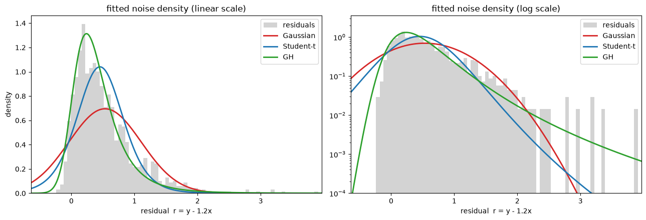
On the linear panel the Gaussian (red) is symmetric and too flat - it misses the tall, asymmetric peak. The Student-t (blue) is more peaked and a little heavier-tailed, but still symmetric. The GH (green) leans into the skew and matches the asymmetric peak best. On the log panel the Gaussian and Student-t right tails fall away while the GH tracks the long, heavy right tail; and where the noise is skewed the differences are starkest - note the GH's short left tail versus the Gaussian's symmetric, data-free left tail.

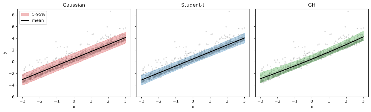
Predictive mean and 5-95% bands

Back in data space: we sample \(p(y \mid x)\) on a grid and take percentiles. Heavy-tailed / skewed models produce wider, asymmetric predictive bands.

xg = np.linspace(-3, 3, 60).reshape(-1, 1)
fig, axes = plt.subplots(1, 3, figsize=(13, 4), sharey=True)
for ax, (name, m) in zip(axes, models.items()):
    samples = m.sample(xg, n_samples=4000)        # (n, n_samples, 1)
    lo, hi = np.percentile(samples[:, :, 0], [5, 95], axis=1)
    ax.scatter(X_train[:, 0], y_train, s=6, alpha=0.2, color='gray')
    ax.fill_between(xg[:, 0], lo, hi, alpha=0.30, color=COLORS[name],
                    label='5-95%')
    ax.plot(xg[:, 0], m.predict(xg), color='k', lw=2, label='mean')
    ax.set_title(name); ax.set_xlabel('x'); ax.set_ylim(-6, 9)
axes[0].set_ylabel('y'); axes[0].legend(loc='upper left')
fig.tight_layout()

Takeaways

• The three regressors are interchangeable in code (fit/predict/sample/score/condition); pick the family that matches your residuals.

• ConditionalStudentTRegressor is the robust choice for heavy tails; ConditionalGHRegressor adds skewness.

• All return a conditional mixture you can sample from or evaluate, and they integrate with scikit-learn pipelines and GridSearchCV like the Gaussian model.

For the mathematics - the densities, the closed-form conditioning, and the EM algorithms - see Distributions & Conditioning.